A single-number yield forecast creates false precision. This is true whether the number comes from USDA WASDE, a private commodity analyst, or a satellite yield model. The USDA August WASDE might say US corn yield is 177.5 bu/acre. That number implies a precision that is not present in the underlying estimation methodology — and for traders making position sizing decisions, that false precision is more dangerous than explicit uncertainty would be. Probability distributions — specifically, the P10/P50/P90 framework — are how satellite yield data should be consumed in commodity trading contexts, and this article explains why and how.
What P10/P50/P90 Actually Represents
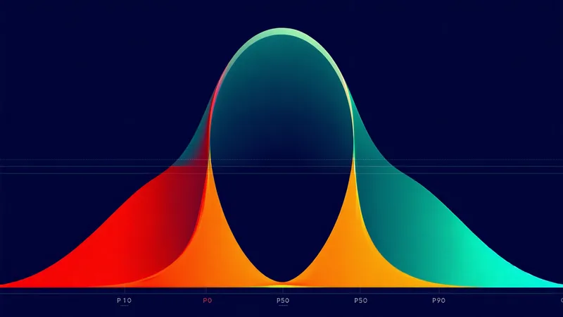
In the terminology used for yield distributions, P50 is the median of the forecast distribution — the yield level that the model assigns 50% probability of being exceeded. P10 is the 10th percentile — the level below which the final yield falls in the worst 10% of scenarios given current season conditions. P90 is the 90th percentile — the level below which yield falls in 90% of scenarios (i.e., the optimistic tail).
A concrete example: on August 5th, with corn in R3-R4 across central Iowa, a satellite yield model might return P10 = 161 bu/acre, P50 = 178 bu/acre, P90 = 192 bu/acre for a specific county. This means the model is saying: there's a 10% chance the county ends the season below 161 bu/acre, a 50% chance it ends below 178 bu/acre, and a 90% chance it ends below 192 bu/acre. The width of the P10-P90 interval (31 bu/acre in this example) quantifies how much uncertainty remains given the crop's current physiological state — which itself reflects the observed NDVI trajectory, weather conditions, and model calibration history.
For a trader, the P50 is not the most important number. The P10 is.
Why the P10 Tail Drives Trading Decisions
Commodity price sensitivity is asymmetric around yield outcomes. A yield outcome at P50 (normal-to-good year) is largely priced into deferred futures contracts well before harvest — the carry structure, basis levels, and storage economics all reflect expected normal supply. What moves price materially is a realized outcome significantly below P50: a drought-year yield realization that reduces national supply below what was priced into the market.
This is why the P10 tail of the yield distribution is the trading-relevant statistic for long corn or short corn positions. The question is not "what is the expected yield?" — that is already in the market at some level — but rather "what is the probability and magnitude of a below-consensus supply outcome, and is the market currently pricing that tail correctly?"
When satellite field data shows a P10 yield for Iowa corn at 161 bu/acre as of August 5th, and the December corn futures market is pricing an implied supply scenario consistent with 175+ bu/acre national average (above our P50), there is a potential mispricing — the options market's implied downside protection may be under-priced relative to what the satellite data says about the distribution's lower tail. Whether that mispricing justifies a specific options strategy depends on many factors beyond satellite yield data, but identifying the gap between market-implied and satellite-derived probability distributions is exactly the analysis that P10/P50/P90 output enables.
Building Yield Scenario Models from Distribution Data
The P10/P50/P90 framework becomes most useful when it is operationalized in a scenario model that connects yield outcomes to price outcomes. A simple scenario structure might look like:
- Base case (P50 scenario): Iowa corn yield of 178 bu/acre, national corn production approximately consistent with August WASDE trend, December corn futures trading at current forward curve.
- Bear supply scenario (P10 scenario): Iowa corn yield of 161 bu/acre; extrapolating similarly stressed conditions across the broader corn belt, national production falls 350-500 million bushels below WASDE base case; December corn futures rally estimated 30-50 cents per bushel based on historical supply-price elasticity in similar deficit years.
- Bull supply scenario (P90 scenario): Iowa corn yield of 192 bu/acre; above-trend national production of 15.2+ billion bushels; end stocks expand, basis weakens, December corn futures under pressure 15-25 cents.
The trading decision — long corn calls, short corn puts, or a combination — is then sized based on: (a) the satellite-derived probability of each scenario, (b) the market's implied pricing of each scenario in options premiums, and (c) the trader's risk tolerance for outcomes outside the P10-P90 range. Scenarios outside P10-P90 — the left tail below P10 — are real but low-probability, and they represent catastrophic loss years (2012 drought) that the market tends to price inadequately until they are clearly developing.
County vs. Regional vs. National: Which Level of Aggregation Matters
One practical question for trading desk applications is the right level of geographic aggregation for yield distributions. County-level P10/P50/P90 is the most granular output — useful for understanding whether a specific supply region is stressed — but it's not directly comparable to national production estimates in WASDE.
The translation from county-level distributions to national production distributions requires weighted aggregation across the full county coverage set: multiply each county's P10/P50/P90 yield by planted acres, sum across counties, and account for the correlation structure between counties (which tend to be positively correlated within a growing season driven by large-scale weather patterns). The last step is non-trivial — simple summation of county P10 yields produces a national P10 that is too pessimistic because it implicitly assumes all counties hit their worst case simultaneously, which is not how crop-area weather events work.
We're not saying county-level distributions require complex correlation modeling before they're useful. For traders with a specific regional position — corn purchased for Illinois delivery, soybeans hedged against eastern Iowa basis — county-level distributions for the specific delivery geography are directly applicable without national aggregation. The national aggregation step is relevant for traders whose position is driven by WASDE-scale US supply surprises; regional traders can use county distributions directly.
The Mid-Season Information Revision: How Distributions Narrow Through the Season
One underappreciated feature of probabilistic yield forecasting is the dynamic of distribution narrowing through the growing season. The P10/P90 spread on June 1st — before significant development has occurred — reflects primarily the climatological range of yield outcomes for that county in a typical year, which might be 40-60 bu/acre for corn. By August 15th, after the crop has moved through pollination and is entering grain fill, the satellite signal has directly observed whether reproductive stress occurred — and the P10/P90 spread narrows to 25-35 bu/acre because many of the uncertain scenarios have been resolved by actual field observations.
For a trader, this narrowing pattern means that the maximum information value from satellite yield distributions is realized in July and early August — the window when uncertainty is still significant (P10/P90 spread 30-40 bu/acre) but enough of the season has been observed to meaningfully distinguish between scenarios (P50 has moved from June trend). This is the period when satellite-derived distributions provide the most alpha relative to WASDE data, and the most relevant comparison to options-implied volatility. Trading desks that evaluate satellite data providers should assess not just the final-season accuracy metrics but the in-season distribution narrowing dynamics — a model that shows slow, late distribution narrowing is providing less trading-relevant information than one that resolves uncertainty quickly as the season progresses.